Transformers - Encoders & Decoders

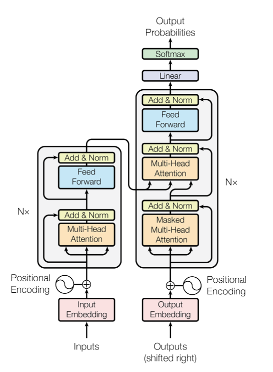
Figure: Transformer encoder-decoder architecture. Source: "Attention Is All You Need" (Vaswani et al., 2017).

🧩 Summary of Flow

Inputs → Embedding → Positional Encoding → Encoder Stack.

Decoder takes shifted outputs → Embedding → Positional Encoding.

Decoder attends to both its own previous outputs and encoder’s outputs.

Final linear + softmax gives output probabilities.

---

This figure illustrates the complete architecture of the Transformer model, a neural network designed for sequence-to-sequence tasks like machine translation. It consists of an encoder on the left and a decoder on the right. The core idea is to process all input tokens in parallel using a mechanism called multi-head attention, which allows the model to weigh the importance of different words in a sequence to each other. This approach eliminates the need for sequential processing, which was a bottleneck in previous models like RNNs.

---

Encoder

The Encoder is on the left and is composed of a stack of identical layers. Its purpose is to process the input sequence and produce a representation of it.

• Input Embedding:

  • The input words are first converted into dense vector representations.

• Positional Encoding:

  • Since the Transformer processes all words simultaneously, it has no inherent sense of word order.
  • The positional encoding adds a vector to each input embedding to give the model information about the position of a word in the sequence.

• Multi-Head Attention:

  • This is the heart of the encoder. It calculates the relationship between all words in the input sequence.
  • For each word, it generates a new representation that is a weighted sum of all other words' representations.
  • The "multi-head" part means this process is done multiple times in parallel, allowing the model to focus on different aspects of the relationships between words.
  Details

  Key, Value, and Query in Attention Function

  In the context of the Transformer's self-attention mechanism, the query, key, and value are concepts derived from retrieval systems and are used to compute the attention scores. All three are vector representations of the same input word, but each plays a different role in the calculation.

  The query ($Q$), key ($K$), and value ($V$) weight matrices are not pre-prepared during pretraining — they are learned during the training process itself.

  Where Q, K, V weights live in the Transformer

  • Each Multi-Head Attention (MHA) block in both the encoder and decoder has:

    • $W_Q$: Query projection matrix
    • $W_K$: Key projection matrix
    • $W_V$: Value projection matrix

  • Locations:

    • Encoder:
      • Self-Attention → Q/K/V weights.
    • Decoder:
      • Self-Attention → Q/K/V weights.
      • Cross-Attention → Another set of Q/K/V weights (because queries come from decoder, keys/values from encoder outputs).

  How They're Created

  1. Initialization

  • When you first create a Transformer model (before any training), the Q, K, V weight matrices are initialized — usually with random values following some distribution (e.g., Xavier/Glorot, Kaiming).
  • This happens once, before training starts, not in the computation/communication loop yet.
  • At this stage, they know nothing about language, vision, etc.

  2. Computation & Communication

  • For each word in the input sequence, its original embedding is transformed into three different vectors: a query (Q), a key (K), and a value (V). This is done by multiplying the word's embedding vector by three separate, trainable weight matrices: $W^Q$, $W^K$, and $W^V$.

    • Query (Q): $Q = \text{Embedding} \times W^Q$
    • Key (K): $K = \text{Embedding} \times W^K$
    • Value (V): $V = \text{Embedding} \times W^V$

    These matrices ($W^Q$, $W^K$, $W^V$) are learned during the model's training.

    Step-by-step in one Transformer block

    (Example: Encoder Self-Attention Block — same logic for decoder’s attention)

    Forward pass → Computation Phase

    1. Input embeddings / hidden states enter the MHA layer.
    2. They are multiplied by $W_Q, W_K, W_V$ to produce Q, K, V vectors:
    $$Q = X W_Q,\quad K = X W_K,\quad V = X W_V$$
    3. Attention scores computed:
    $$\text{Attention}(Q, K, V) = \text{softmax}\left(\frac{QK^T}{\sqrt{d_k}}\right) V$$
    4. Output flows to residual connection + layer norm, then to the MLP (Feed-Forward Network).

    At this point:
    ✅ Computation phase — but no weights are updated yet, just activations produced.

    ---

    Backward pass → Computation + Communication Phase

    5. Loss computed (at the end of the model).

    6. Backpropagation starts:

       • Gradients flow back through MLP, then through attention outputs, then into Q, K, V computations.
       • Gradients for $W_Q, W_K, W_V$ are calculated here (computation phase).

    7. If distributed training:

       • Gradients for $W_Q, W_K, W_V$ are communicated across devices (all-reduce operation).
       • This is the communication phase — ensures all GPUs/nodes have the same gradients.

    ---

    Optimizer step → Computation Phase

    8. The optimizer (e.g., Adam) updates $W_Q, W_K, W_V$ using their synchronized gradients.
    9. Updated weights are stored for the next forward pass.

    ---

  3. Summary Table — Q/K/V Weight Updates in Transformer Blocks

  Transformer Block	Where Q/K/V Live	When Gradients Computed (Computation)	When Gradients Synced (Communication)	When Weights Updated
  Encoder Self-Attn	Inside MHA	Backward pass through self-attn	After backprop, before optimizer step	Optimizer step
  Decoder Self-Attn	Inside MHA	Backward pass through self-attn	Same	Same
  Decoder Cross-Attn	Inside MHA	Backward pass through cross-attn	Same	Same

  What They Do

  The core idea is to think of the attention mechanism as a search process.

  • Query: The query is the vector representing the current word you are focused on. It's what you are "searching" with. For example, if you are calculating the attention output for the word "it," your query vector will be for "it."
  • Keys: The keys are the vectors for all the words in the sequence. They represent what you are "searching against." Each key is used to determine how relevant its corresponding word is to the query word.
  • Values: The values are also vectors for all the words in the sequence. The value vectors, on the other hand, are the vectors that contain the information that will be used to form a new representation for the current word. They are the actual "payload" of the attention mechanism.

  ---

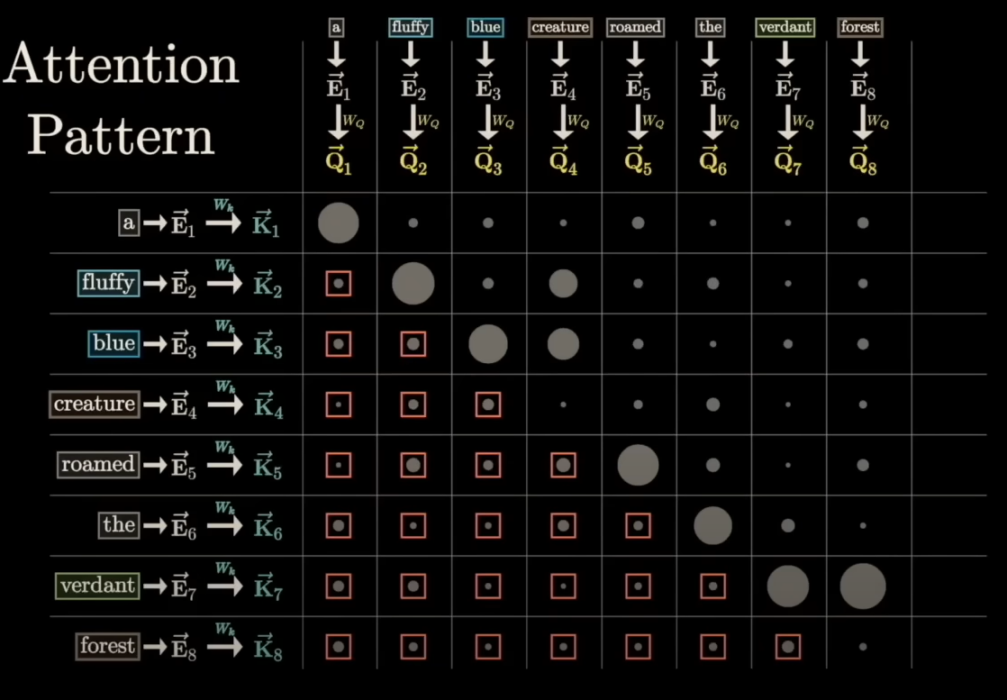
  How the attention mechanism works

  The core formula for scaled dot-product attention is:

  $$\text{Attention}(Q, K, V) = \text{Softmax}\left(\frac{Q K^\top}{\sqrt{d_k}}\right) V$$

  Step-by-step:

  1. Matching stage (Q and K)

  • For each position $i$ (Query), we compute a similarity score with every position $j$ (Key) using a dot product:

    $$\text{score}(i, j) = Q_i \cdot K_j$$

  • These scores tell us how much attention position $i$ should pay to position $j$.

  2. Softmax to get weights

  • The scores are scaled by $\frac{1}{\sqrt{d_k}}$ to stabilize gradients.

  • A softmax is applied across all $j$ for a given $i$, producing attention weights $\alpha_{ij}$:

    $$\alpha_{ij} = \frac{\exp(\text{score}(i, j))}{\sum_k \exp(\text{score}(i, k))}$$

  Attention weights are intermediate results inside the Attention block, just before being multiplied by the value vectors $V$.
  Attention weights are updated at Every forward pass and depend on current $Q$ and $K$, so they change with input and layer state. They are not stored as part of model weights; they disappear after computation.

  Relationship Between $K$/$Q$/$V$ weights and Attention weights

  Feature	Key/Query/Value Weight Matrices	Attention Weights (Softmax Output)
  Type	Learned parameters	Computed activations
  Persistence	Stored in model and updated during training	Temporary, discarded after forward pass
  Location	Inside Attention block (parameter matrices)	Inside Attention block (computed output)
  Phase Updated	Computation phase during training	Computed fresh every forward pass
  Function	Transform inputs into Q, K, V vectors	Decide "who attends to whom"

  • Now, each weight says: “How much of token $j$’s content should be sent to token $i$?”

  3. Using the Values (V)

  • Finally, the Values hold the actual content vectors we want to aggregate.

  • For each position $i$, we take a weighted sum of all Value vectors $V_j$ using the attention weights:

    $$\text{output}_i = \sum_j \alpha_{ij} \cdot V_j$$

  • This output is a contextualized representation of token $i$, because it blends information from other tokens according to relevance.

  • This means:

    • If $\alpha_{ij}$ is high, token $i$ borrows a lot from token $j$’s information $V_j$.
    • If $\alpha_{ij}$ is low, token $i$ mostly ignores $V_j$.

  • Why Values matter

    • Keys are just for matching.

    • Values are what actually gets transferred.

    • The “relevance” comes from $\alpha_{ij}$, and the “context” comes from pulling in pieces of $V_j$ for all $j$.

    • In theory, Q and K could be identical to V, but separating them allows the model to decide different ways to match and different content to pass along.

    • For example:

      • Keys might encode syntactic roles.
      • Values might carry semantic content.

  • An Analogy: Library Search

    Imagine you're at a library looking for books on a specific topic.

    • Query: Your search query (e.g., "History of AI") is the query vector.
    • Keys: The labels or keywords on all the books in the library (e.g., "Computer Science," "Robotics," "1960s") are the key vectors.
    • Values: The actual content of each book is the value vector.

    You match your query against all the keys. Books with keys that closely match your query get a high relevance score. Then, you use these scores to decide how much "information" (value) from each book you should "read" to form a comprehensive answer. The Transformer's self-attention mechanism works similarly, but it does this for every word in the sequence simultaneously.

  4. Linear Projection (Post-Attention)

  • In a Transformer implementation, this new weighted-sum vector goes through a final linear layer (sometimes called $W_O$) to mix the multiple attention heads’ results into one representation per token.
  • Formula (simplified for one head):

  $$Z_i = \left( \sum_j \alpha_{ij} \cdot V_j \right) W_O$$

  • If there are multiple heads, all head outputs are concatenated before multiplying by $W_O$.

  5. Residual Connection

  • The Transformer adds the original input embedding (the one that was used to create $Q, K, V$) back to the attention output:

    $$\text{AttnOutput}_i = \text{Input}_i + Z_i$$

    This residual connection helps preserve the original token information while allowing the model to integrate the contextualized representation.

  6. Layer Normalization

  • After the residual sum, LayerNorm is applied to stabilize and normalize the representation:

    $$\text{NormOutput}_i = \text{LayerNorm}(\text{AttnOutput}_i)$$

  7. Feed-Forward Network (MLP)

  • The normalized vector is then sent to the position-wise feed-forward network (two linear layers with a nonlinearity like GELU/ReLU):

    $$\text{FFNOutput}_i = \text{MLP}(\text{NormOutput}_i)$$

  • Another residual connection + LayerNorm happens after this MLP.

• Add & Norm:

  • A residual connection (the "Add" part) adds the input of the sub-layer to its output, and then the result is passed through a layer normalization (the "Norm" part).
  • This helps with training by preventing the gradients from vanishing.
  Details

  Residual Connection (The "Add" Part)

  A residual connection is a shortcut that connects the input of a sub-layer directly to its output. In the Transformer, for any sub-layer $Sublayer(x)$, the output is calculated as:

  $$x + Sublayer(x)$$

  By allowing the gradient to flow directly through this "shortcut," it helps to mitigate the vanishing gradient problem. Without residual connections, the gradients could become extremely small as they are backpropagated through many layers, making it difficult to train the model effectively. This allows the network to learn a sub-layer's function as a modification to its input, rather than having to learn the entire transformation from scratch.

  ---

  Layer Normalization (The "Norm" Part)

  Following the residual connection, the result is passed through a layer normalization step. This component normalizes the activations across the features for each individual sample in the batch. Specifically, it computes the mean and variance of the activations within a single layer for a given input sequence and then uses these statistics to normalize the values.

  $$LayerNorm(x) = \gamma \odot \frac{x - \mu}{\sqrt{\sigma^2 + \epsilon}} + \beta$$

  Here, $\mu$ and $\sigma$ are the mean and standard deviation of the input values across the features, and $\gamma$ and $\beta$ are learnable parameters that allow the network to "undo" the normalization if it determines that this is a better configuration.

  The primary benefits of layer normalization are:

  • Faster and More Stable Training: It stabilizes the learning process by ensuring that the inputs to each sub-layer are within a consistent range, regardless of the previous layers' outputs.
  • Reduced Dependence on Learning Rate: Layer normalization makes the network less sensitive to the choice of the learning rate, which simplifies the tuning of hyperparameters.

  In essence, the combination of Add & Norm ensures that the deep Transformer architecture can be trained effectively by creating a direct path for gradient flow and stabilizing the activations within each layer.

• Feed Forward (Aka MLP- Multi-Layer Perceptron):

  • A simple, fully connected neural network is applied to each position separately and identically.
  • Typically two linear layers with a ReLU in between.
  • The MLP injects non-linearity and feature transformation into the model, enabling it to learn more complex mappings at each position.

🔁 This whole block is repeated N times (e.g., 6 in the base model).

---

Decoder

The Decoder is on the right and also consists of a stack of identical layers. Its job is to generate the output sequence one token at a time. It receives the encoder's output and the previously generated output tokens as input.

• Output Embedding & Positional Encoding:
  • Similar to the encoder, the previously generated output words are embedded, and positional information is added.
  • Inputs are shifted right so that predictions can’t “see the future.”
• Masked Multi-Head Attention:
  • This is a crucial difference. It's the same as the encoder's multi-head attention but with a "mask" applied. The mask ensures that the model can only attend to the words it has already generated (to preserve autoregressive decoding).
  • Before applying the softmax, set the next/future tokens to $-\infty$ (After it passes through the softmax function, that becomes zero).
  • This prevents it from "cheating" by looking at future words in the output sequence during training.
• Encoder-Decoder Attention:
  • After the masked attention layer, a second multi-head attention layer takes the output from the decoder's masked attention layer and the final output from the encoder stack.
  • This layer allows the decoder to focus on relevant parts of the input sequence (like attention in seq2seq models) while generating the next word, which is essential for tasks like translation.
• Add & Norm and Feed Forward:
  • These layers function identically to their counterparts in the encoder, further refining the decoder's representation.
• Linear & Softmax:
  • The final output of the decoder stack is a vector that is fed into a linear layer, which projects it into a larger vector called a logit vector. This logit vector is the size of the vocabulary.
  • The softmax layer then converts these logits into probabilities, indicating the likelihood of each word in the vocabulary being the next word in the output sequence.
  • The word with the highest probability is chosen as the final output.

---

💡 Key Components Highlighted in the Diagram

Component	Description
Multi-Head Attention	Allows the model to attend to different parts of the sequence in parallel.
Masked Multi-Head Attention	Prevents a position from attending to future positions.
Feed Forward	Two-layer FFN applied to each position independently.
Add & Norm	Residual connection followed by layer normalization.
Positional Encoding	Added to embeddings to encode order of tokens.
Softmax	Converts output logits to probabilities.

---

Cases where only decoders are used

1. Autoregressive Language Modeling

• Goal: Predict the next token given all previous tokens.

• Why decoder-only?

  • The model sees only the tokens generated so far.
  • Masked self-attention enforces the “no peeking ahead” rule.

• Examples:

  • GPT, GPT-2, GPT-3, GPT-4 — large language models for text generation, code generation, and chat.
  • OpenAI Codex, LLaMA, MPT, Falcon, etc.

2. Text Generation Without Separate Input Sequence

• Goal: Produce free-form text from a prompt or initial context.

• Why decoder-only?

  • The "prompt" is treated as the first part of the output sequence.
  • No need for an encoder because there’s no separate source sequence to encode.

• Examples:

  • Story generation, poetry, summarization (prompt-based).
  • InstructGPT-style models where instructions are part of the input text.

3. Single-Stream Tasks

• Goal: Process input and output in a single stream (one continuous sequence).

• Why decoder-only?

  • Input and output are concatenated in one sequence.
  • Masking ensures that output tokens can’t see future output tokens, but can see all input tokens (since they appear before them in the sequence).

• Examples:

  • Prompt-based question answering without separate encoding stage.
  • Few-shot in-context learning (the examples + question are just part of the sequence).

Key Difference from Encoder–Decoder

• Encoder–Decoder: Needed when there’s a source sequence and a target sequence (e.g., translation: French → English). The encoder processes the source, and the decoder generates the target conditioned on the source.

• Decoder-Only: Suitable when:

  1. The model generates based on what it has already generated.
  2. Input and output share the same token stream.
  3. There’s no need for a separate encoded representation.

💡 Rule of thumb:

• If you have an input sequence separate from the output sequence → use encoder–decoder.
• If your task is just to generate a continuation of a sequence → use decoder-only.

---

Online sources:

• Stanford CS25: V2 I Introduction to Transformers w/ Andrej Karpathy

• Visualizing transformers and attention | Talk for TNG Big Tech Day '24